Brave Rats: First Turn Analysis

First turn analysis based on human data

Welcome to an analysis of Brave Rats statistics, with real data collected from real players. Brave Rats is a micro card game designed by Seiji Kanai. This is the first in a series of posts about this game, as I seek to use traditional AI, deep learning, and more data to delve deeper into the strategy of this seemingly simple simultaneous move war game. If you’re not familiar with the game, I recommend this 5-minute video tutorial to best be able to understand.

As of writing this commentary, I have recorded 62 games, mostly but not always with myself as one of the players. After removing two tied games, this gives a total of 120 opening moves to analyze. The first turn, as in many games, is very important yet very abstract and hard to make concrete statements about as it is so far removed from the end state of the game. This analysis will attempt to provide some data-driven guidance to this stage of play.

# Importing the data and mirroring it

columnNames = c("Game #","Player 1","Player 2", "P2 wins?",  "Notes", "P1 Card 1","P2 Card 1","P1 Card 2","P2 Card 2","P1 Card 3","P2 Card 3","P1 Card 4","P2 Card 4","P1 Card 5","P2 Card 5","P1 Card 6","P2 Card 6","P1 Card 7","P2 Card 7","P1 Card 8","P2 Card 8") %>% 
  str_replace_all("[ #?]", "")
ratData <- read_csv("Brave Rats Data - Record.csv", 
                    skip_empty_rows = TRUE, 
                    col_names = columnNames, 
                    skip=1)%>% 
  select(P2wins, P1Card1, P2Card1)

notFlipped <- ratData %>% 
  mutate(P1Wins = abs(P2wins-1), P1Card = ratData$P1Card1, P2Card = ratData$P2Card1) %>% select(P1Wins, P1Card, P2Card)

flipped <- ratData %>% 
  mutate(P1Wins = P2wins, P1Card = ratData$P2Card1, P2Card = ratData$P1Card1) %>% select(P1Wins, P1Card, P2Card)

fullSet <- rbind(notFlipped, flipped) %>% 
  filter(P1Wins != 0.5) %>% 
  mutate(Outcome = ifelse(  P1Wins==1, "Win", "Loss"),
    Outcome = factor(Outcome, levels = c("Loss", "Win")))

We’ll start with the overall distribution of first cards played and their win rates:

# To make this plot exactly how I want, I first tabulate the statistics and labels I'll be using for each card, then input them into ggplot.
fullSet %>% 
  group_by(P1Card, Outcome) %>% 
  summarize(count = n()) %>% 
  group_by(P1Card) %>% 
  pivot_wider(names_from = Outcome, values_from = count, values_fill = 0) %>% # Pivot wider then longer to create "0" rows where there were previously no rows.
  pivot_longer(c(Loss, Win), names_to = "Outcome", values_to = "count") %>% 
  mutate(proportion = count / sum(count),
         percent = if_else(Outcome == "Loss", "", str_c(round(proportion, 3)*100, "%"))) %>%
  ungroup() %>% 
  mutate(card_prop = count / sum(count)) %>% 
  ggplot(aes(x = P1Card, y = card_prop, fill = Outcome)) +
  geom_bar(stat = "identity") +
  geom_text(aes(label = percent), vjust = -0.2, position = "stack") +
  ggtitle("Frequency of use and win rate of each starting card") +
  scale_x_continuous(breaks = c(0,1,2,3,4,5,6,7)) +
  scale_y_continuous(labels = scales::percent) +
  ylab("Percent of games (n = 120)") +
  xlab("Card")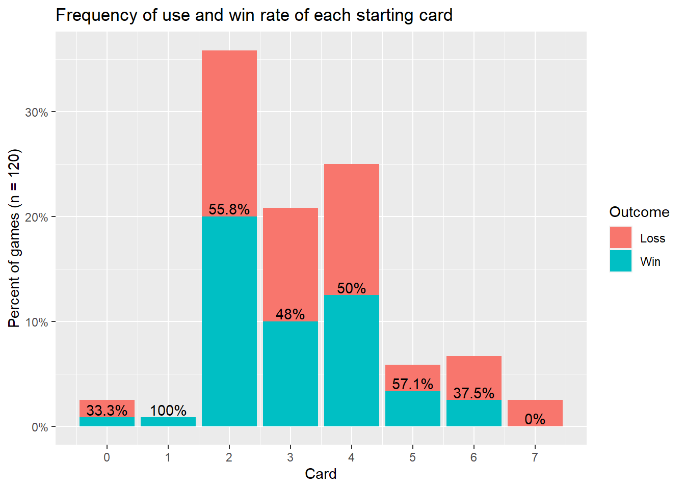

The clear trend is that only 3 cards, Spy(2), Assassin(3), and Ambassador(4) are by far the frequent starting cards. With Spy(2) being played over 40% of the time, you’d think Ambassador(4) would be very good, giving its user a 40% chance to start off with 2 points by beating the spy. We will explore this interaction in more depth later. Wizard(5) has the highest win rate currently, winning 4/7 times. This makes sense because it beats all 3 of the most common starters, so with some further gameplay we could quickly find it to be a viable starter.

While it’s easy to find the cards that are most likely to score a point on the first round, the further consequences of playing them can be counterintuitive. Since using one’s best cards will make it hard to win future rounds, our current strategies emphasize starting with some of the lowest cards. The table below shows the outcomes of each combination of the most common starters (other combinations had sample sizes too low for meaningful analysis).

fullSet %>% 
  filter(P1Card %in% c(2,3,4) & P2Card %in% c(2,3,4)) %>% 
  mutate(P2Card=factor(P2Card, levels=c("4","3","2"))) %>% 
  ggplot(aes(x=Outcome, fill=Outcome)) +
  geom_bar(aes(stat="count")) +
  facet_grid(vars(P2Card), vars(P1Card), switch="both") +
  ylab("Opponent's Card") +
  xlab("Your Card")+
  theme(axis.text.x = element_blank()) +
  scale_y_continuous(breaks = seq(0,100, 2)) +
  ggtitle("Outcomes for each first turn matchup")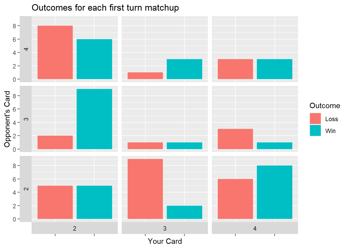

This last graph may be somewhat jarring, so I’ll explain how to read it. On the X is what card you picked, and on the Y is the card your opponent picked. At each intersection is a small plot, showing the history of wins and losses in games that started that way. Immediately apparent is one of the major reasons why the Spy(2) has been so successful. In games against Assassin(3), the Spy(2) player has won 9 out of 11 times. Also surprisingly, even in what seems to be an extremely favorable situation of playing Ambassador(4) against Spy(2), thereby gaining 2 victories, the Spy player has actually won 6 out of the 14 games.

Of course, with sample sizes this small after dividing up every common matchup, nothing is proven. Nevertheless, I hope this can inform better strategies to test these conclusions in the field of battle.